
Generative models represent a wide class of systems that are able to create new samples which follow some training distribution. Variational Autoencoders (VAEs) are an example of these models which are trained through a bottleneck latent space, forcing the model to learn meaningful representations of its inputs.
In this article we’ll train a simple VAE to reconstruct rectangular objects and investigate the latent space it learns.
The Dataset
We’ll define a simple generator which creates rectangles of one of 9 colours on a 10x10 black background. The rectangles can be of arbitrary size and are placed somewhere in the grid. This gives us examples as seen below. For training, we generate 1000 samples.
The Model
For an in-depth dive into VAEs you can find many good tutorials on the web. The key insight for our purpose is that they’re made of two key parts: the encoder and the decoder. The encoder will take our rectangle images and convert them from ‘image space’ to some lower dimensional ‘latent space’. Similarly, the decoder takes a latent representation and converts it back to an image.
Given we’re working with images, we model the encoder as a convolutional neural network (CNN) with a couple of layers followed by a fully connected layer. The decoder uses the convolutional transpose layer to achieve the reverse operation. Additionally, we’ll be using discrete colours, so we’ll utilise embeddings to convert our colours to an embedding representation.
The latent space and model can be quite small since the problem is very simple. We use an embedding size of 4, a latent size of 8 and filter sizes of 16 and 32. This yields a small model of 20,000 parameters.
Model Architecture:
ConvVAE(
  (embedding): Embedding(10, 8)
  (encoder): Sequential(
    (0): Conv2d(8, 4, kernel_size=(3, 3), stride=(1, 1), padding=(1, 1))
    (1): ReLU()
    (2): Conv2d(4, 8, kernel_size=(3, 3), stride=(1, 1), padding=(1, 1))
    (3): ReLU()
  )
  (fc_mu): Linear(in_features=800, out_features=8, bias=True)
  (fc_logvar): Linear(in_features=800, out_features=8, bias=True)
  (fc_decode): Linear(in_features=8, out_features=800, bias=True)
  (decoder): Sequential(
    (0): ConvTranspose2d(8, 4, kernel_size=(3, 3), stride=(1, 1), padding=(1, 1))
    (1): ReLU()
    (2): ConvTranspose2d(4, 10, kernel_size=(3, 3), stride=(1, 1), padding=(1, 1))
  )
)
Training
For training we can follow the standard practices. We use Adam with a learning rate of 0.001 for optimisation and run for 1000 epoch. We use the standard loss functions for VAE which is a combination of the reconstruction loss (how well we can reconstruct the image) and the KL divergence (how well our data samples match a prior normal distribution). The training results are below. The model showed good improvements, though could likely be trained for longer.
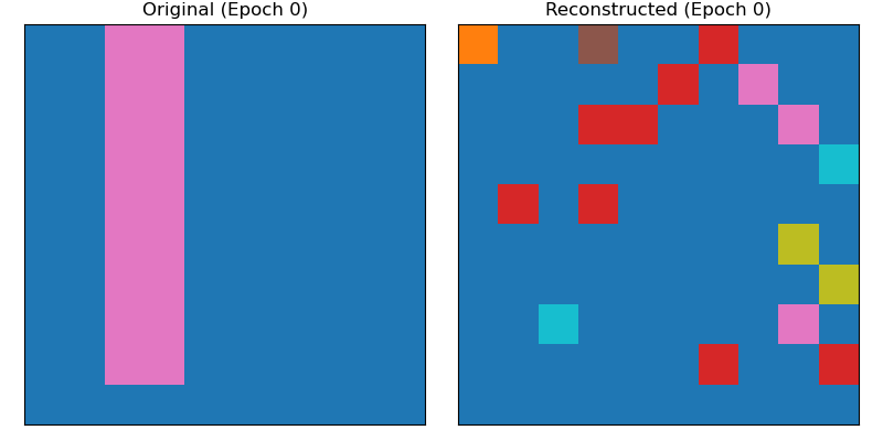
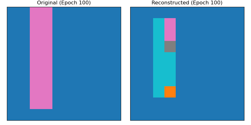
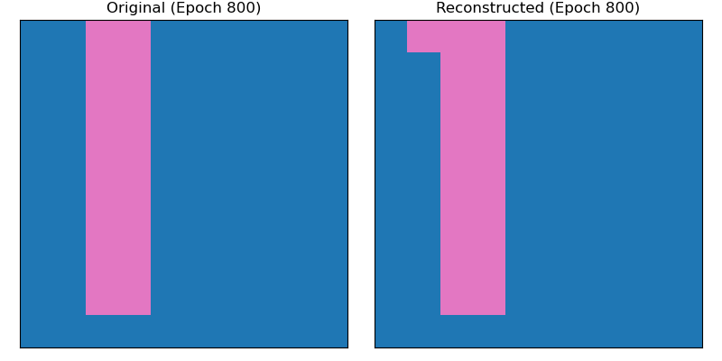
Epoch 0: Loss = 2.2118 (Recon: 2.1934, KL: 0.0184) Epoch 100: Loss = 0.8559 (Recon: 0.7493, KL: 0.1065) Epoch 200: Loss = 0.8190 (Recon: 0.6984, KL: 0.1206) Epoch 300: Loss = 0.3672 (Recon: 0.1962, KL: 0.1709) Epoch 400: Loss = 0.2572 (Recon: 0.0850, KL: 0.1722) Epoch 500: Loss = 0.2313 (Recon: 0.0596, KL: 0.1717) Epoch 600: Loss = 0.2207 (Recon: 0.0511, KL: 0.1696) Epoch 700: Loss = 0.2152 (Recon: 0.0479, KL: 0.1674) Epoch 800: Loss = 0.2116 (Recon: 0.0447, KL: 0.1669) Epoch 900: Loss = 0.2114 (Recon: 0.0449, KL: 0.1665)
The images below show the same sample at different steps during training. Initially the model predicts random noise, then learns to map the background area well before finally getting the shape mostly correct. I noticed that the model struggles to reduce the small errors, often getting just one pixel wrong, one extra or one less.
Latent Space Exploration
Now that we have a trained model we can explore the latent space to see if it’s learning meaningful representations. So what would expect the latent space to represent? For one, we’d expect colour to be a useful feature in that space. So if I tweak the value of one dimension (or two), then the colour of the output should change while everything else remains relatively fixed.
To investigate this, we can first build a features dataset and then see how these features change with the latent space. Features can be directly calculated when we generate our images.
Firstly, let’s look at colour. We create a table which consists of the latent space vector and its corresponding colour (e.g. 7, 0.21, -0.10, 0.99, …). One way to look at which column controls colour is to then look at which latent column varies the most between colours. For example, the latent might be an average of 0.3 for blue and an average of -0.7 for red, indicating it is predictive of the colours.
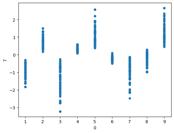
Using this method we see clearly how dimension 7 represents colour with values tightly clustered for each colour. Similarly, we see that for the first row that a rectangle appears in is highly correlated with the first dimension. Interestingly, it’s roughly linear, flipping around the middle.
Given we now know what the latent values correspond to, we can try editing our latents directly to influence the outputs. We choose the latent dimension which varies with height and apply modifications to the latent of a short rectangle. We first extract the latent using the model’s encoder, we then directly edit the latent dimension by some small amount (rescaling the other values to keep the norm constant). Finally, we can visualise the output by using our decoder and see how it changes with the amount we edit.
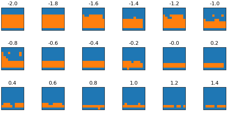
The figure below shows that while the model hasn’t well learnt to stay on the manifold of coloured rectangles it is clearly increasing and decreasing the height of the object as the value of the latent changes. This tells us that the model has learnt meaningful representations in its latent space.
What’s Next
With our trained model we can now do a few things.
- We could ‘edit’ objects by tuning their latent representations as we saw.
- We could generate new objects by sampling from the normal distribution directly and passing that latent vector into our decoder.
- We could train a more useful model on top of our encoder model. For example, with just a few labelled samples of e.g. the colour, we could add a layer on top of our encoder and train a model that can discriminate between them. Because we’ve already got a good representation with our model, we can use just a few labelled samples.
Summary
This experiment demonstrates how even a simple VAE can learn to reconstruct structured pixel patterns and capture meaningful features in its latent space. Through training, the model progresses from noise to accurate reconstructions, and its latent dimensions emerge as interpretable axes controlling attributes such as colour and height. While the model is not perfect—it still struggles with small pixel-level errors—it nonetheless illustrates the power of generative models to compress and disentangle information. Beyond reconstruction, this foundation opens up possibilities for editing, controlled generation, and downstream tasks with limited supervision, showing how VAEs can serve as versatile tools for both analysis and creativity.